机器学习Python教程
简介
 在上一章中,我们使用纯 Python 实现了一个简单的 感知器 (Perceptron) 类。
sklearn 模块也包含一个 Perceptron 类。我们了解到感知器是一种解决二元分类 (binary classifier) 问题的算法。这意味着感知器是一个二元分类器,可以判断输入是属于某一类还是另一类,例如“垃圾邮件”或“非垃圾邮件”。我们通过将权重与特征向量(即输入)进行线性组合来实现这一点。
令人惊奇的是,感知器算法早在 1958 年就由 Frank Rosenblatt 发明了。该算法是在定制的硬件上实现的,被称为“Mark 1 感知器”。这个硬件是为图像识别而设计的。
这项发明曾被极度高估:1958 年,《纽约时报》在 Rosenblatt 的新闻发布会后写道:“海军新设备通过实践学习;心理学家展示了旨在阅读和变得更聪明的计算机雏形”。
最初看起来非常有前景的东西,很快就被证明无法兑现其承诺。这些感知器无法被训练识别多种模式类别。
示例:感知器类
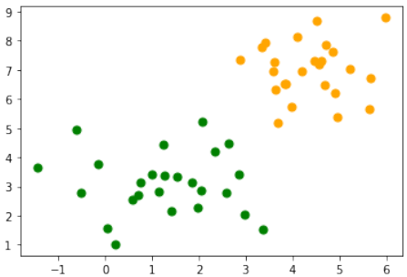
我们将借助 make_blobs 创建一个二元测试集:
import matplotlib.pyplot as plt
from sklearn.datasets import make_blobs

n_samples = 50
data, labels = make_blobs(n_samples=n_samples,
centers=([1.1, 3], [4.5, 6.9]),
random_state=0)

colours = ('green', 'orange')
fig, ax = plt.subplots()

for n_class in range(2):
    ax.scatter(data[labels==n_class][:, 0],
    data[labels==n_class][:, 1],
    c=colours[n_class],
    s=50,
    label=str(n_class))
我们将测试集分成训练集和测试集:
from sklearn.model_selection import train_test_split

datasets = train_test_split(data,
labels,
test_size=0.2)
train_data, test_data, train_labels, test_labels = datasets
我们将使用 sklearn.linear_model 中的 Perceptron 类:
from sklearn.linear_model import Perceptron

p = Perceptron(random_state=42)
p.fit(train_data, train_labels)
输出:Perceptron(random_state=42)
我们可以计算训练集和测试集上的预测并评估得分:
from sklearn.metrics import accuracy_score

predictions_train = p.predict(train_data)
predictions_test = p.predict(test_data)

train_score = accuracy_score(predictions_train, train_labels)
print("score on train data: ", train_score)

test_score = accuracy_score(predictions_test, test_labels)
print("score on test data: ", test_score) # 修正原文中的"score on train data"
输出:
score on train data: 1.0
score on test data: 0.9
p.score(train_data, train_labels)
输出:1.0
使用感知器分类器对鸢尾花数据进行分类
我们希望将感知器分类器应用于鸢尾花数据集,该数据集我们已在关于 k-近邻 (k-nearest neighbor) 的章节中使用过。
加载鸢尾花数据集:
import numpy as np
from sklearn.datasets import load_iris

iris = load_iris()
我们有一个问题:感知器分类器只能用于二元分类问题,但鸢尾花数据集包含三个不同的类别,即“setosa”、“versicolor”、“virginica”,分别对应标签 0、1 和 2:
iris.target_names
输出:array(['setosa', 'versicolor', 'virginica'],
dtype='<U10')
我们将“versicolor”和“virginica”类别合并为一个类别。这意味着只剩下两个类别。因此,我们可以使用分类器区分:
-
鸢尾花 setosa
-
非鸢尾花 setosa,换句话说,是“virginica”或“versicolor”
我们通过以下命令实现这一点:
targets = (iris.target==0).astype(np.int8)
print(targets)
输出:
[1 1 1 1 1 1 1 1 1 1 1 1 1 1 1 1 1 1 1 1 1 1 1 1 1 1 1 1 1 1 1 1
1 1 1 1 1
1 1 1 1 1 1 1 1 1 1 1 1 1 0 0 0 0 0 0 0 0 0 0 0 0 0 0 0 0 0 0 0
0 0 0 0 0
0 0 0 0 0 0 0 0 0 0 0 0 0 0 0 0 0 0 0 0 0 0 0 0 0 0 0 0 0 0 0 0
0 0 0 0 0
0 0 0 0 0 0 0 0 0 0 0 0 0 0 0 0 0 0 0 0 0 0 0 0 0 0 0 0 0 0 0 0
0 0]
我们将数据分为训练集和测试集:
from sklearn.model_selection import train_test_split

datasets = train_test_split(iris.data,
targets,
test_size=0.2)
train_data, test_data, train_labels, test_labels = datasets
现在,我们创建一个 Perceptron 实例并拟合训练数据:
from sklearn.linear_model import Perceptron

p = Perceptron(random_state=42,
max_iter=10,
tol=0.001)
p.fit(train_data, train_labels)
输出:Perceptron(max_iter=10, random_state=42)
现在,我们准备进行预测,我们将查看一些随机选择的 X 值:
import random

sample = random.sample(range(len(train_data)), 10)
for i in sample:
    print(i, p.predict([train_data[i]]))
输出示例:
99 [1]
50 [0]
57 [0]
92 [0]
54 [0]
64 [0]
108 [0]
47 [0]
34 [0]
89 [0]
from sklearn.metrics import classification_report

print(classification_report(p.predict(train_data), train_labels))
输出:
              precision    recall  f1-score   support

           0       1.00      1.00      1.00        76
           1       1.00      1.00      1.00        44

    accuracy                           1.00       120
   macro avg       1.00      1.00      1.00       120
weighted avg       1.00      1.00      1.00       120
from sklearn.metrics import classification_report

print(classification_report(p.predict(test_data), test_labels))
输出:
              precision    recall  f1-score   support

           0       1.00      1.00      1.00        24
           1       1.00      1.00      1.00         6

    accuracy                           1.00        30
   macro avg       1.00      1.00      1.00        30
weighted avg       1.00      1.00      1.00        30
INTRODUCTION
In the previous chapter, we had
implemented a simple Perceptron class
using pure Python. The module
sklearn contains a Perceptron
class. We saw that a perceptron is an
algorithm to solve binary classifier
problems. This means that a Perceptron is
abinary classifier, which can decide
whether or not an input belongs to one or
the other class. E.g. "spam" or "ham". We
accomplished this by linearly combining
weights with the feature vector, i.e. the
input.
It is amazing that the perceptron algorithm was already invented in the year 1958 by Frank Rosenblatt. The
algorithm was implemented in custom-built hardware, called "Mark 1 perceptron". This hardware was
designed for image recognition.
The invention has been extremely overestimated: In 1958 the New York Times wrote after a press conference
with Rosenblatt: "New Navy Device Learns By Doing; Psychologist Shows Embryo of Computer Designed to
Read and Grow Wiser"
What initially seemed very promising was quickly proved incapable of keeping its promises. Thes perceptrons
could not be trained to recognise many classes of patterns.
EXAMPLE: PERCEPTRON CLASS
We will create with the help of make_blobs a binary testset:
import matplotlib.pyplot as plt
from sklearn.datasets import make_blobs
n_samples = 50
data, labels = make_blobs(n_samples=n_samples,
centers=([1.1, 3], [4.5, 6.9]),
random_state=0)
colours = ('green', 'orange')
fig, ax = plt.subplots()
136
for n_class in range(2):
ax.scatter(data[labels==n_class][:, 0],
data[labels==n_class][:, 1],
c=colours[n_class],
s=50,
label=str(n_class))
We will split our testset into a learnset and testset:
from sklearn.model_selection import train_test_split
datasets = train_test_split(data,
labels,
test_size=0.2)
train_data, test_data, train_labels, test_labels = datasets
We will use not the Perceptron class of sklearn.linear_model :
from sklearn.linear_model import Perceptron
p = Perceptron(random_state=42)
p.fit(train_data, train_labels)
Output:Perceptron(random_state=42)
We can calculate predictions on the learnset and testset and can evaluate the score:
from sklearn.metrics import accuracy_score
predictions_train = p.predict(train_data)
137
predictions_test = p.predict(test_data)
train_score = accuracy_score(predictions_train, train_labels)
print("score on train data: ", train_score)
test_score = accuracy_score(predictions_test, test_labels)
print("score on train data: ", test_score)
score on train data:
1.0
score on train data:
0.9
p.score(train_data,Output:1.0
train_labels)
CLASSIFYING THE IRIS DATA WITH PERCEPTRON CLASSIFIER
We want to apply the Perceptron classifier on the iris dataset, which we had already used in our chapter
on k-nearest neighbor
Loading the iris data set:
import numpy as np
from sklearn.datasets import load_iris
iris = load_iris()
We have one problem: The Perceptron classifiert can only be used on binary classification problems, but
the Iris dataset consists fo three different classes, i.e. 'setosa', 'versicolor', 'virginica', corresponding to the
labels 0, 1, and 2:
iris.target_names
Output:array(['setosa', 'versicolor', 'virginica'], dtype='<U10')
We will merge the classes 'versicolor' and 'virginica' into one class. This means that only two classes are left.
So we can differentiate with the classifier between
• Iris setose
• not Iris setosa, or in other words either 'viriginica' od 'versicolor'
We accomplish this with the following command:
targets = (iris.target==0).astype(np.int8)
print(targets)
138
[1 1 1 1 1 1 1 1 1 1 1 1 1 1 1 1 1 1 1 1 1 1 1 1 1 1 1 1 1 1 1 1
1 1 1 1 1
1 1 1 1 1 1 1 1 1 1 1 1 1 0 0 0 0 0 0 0 0 0 0 0 0 0 0 0 0 0 0 0
0 0 0 0 0
0 0 0 0 0 0 0 0 0 0 0 0 0 0 0 0 0 0 0 0 0 0 0 0 0 0 0 0 0 0 0 0
0 0 0 0 0
0 0 0 0 0 0 0 0 0 0 0 0 0 0 0 0 0 0 0 0 0 0 0 0 0 0 0 0 0 0 0 0
0 0 0 0 0
0 0]
We split the data into a learn and a testset:
from sklearn.model_selection import train_test_split
datasets = train_test_split(iris.data,
targets,
test_size=0.2)
train_data, test_data, train_labels, test_labels = datasets
Now, we create a Perceptron instance and fit the training data:
from sklearn.linear_model import Perceptron
p = Perceptron(random_state=42,
max_iter=10,
tol=0.001)
p.fit(train_data, train_labels)
Output:Perceptron(max_iter=10, random_state=42)
Now, we are ready for predictions and we will look at some randomly chosen random X values:
import random
sample = random.sample(range(len(train_data)), 10)
for i in sample:
print(i, p.predict([train_data[i]]))
139
99 [1]
50 [0]
57 [0]
92 [0]
54 [0]
64 [0]
108 [0]
47 [0]
34 [0]
89 [0]
from sklearn.metrics import classification_report
print(classification_report(p.predict(train_data), train_labels))
precision
recall
f1-score
support
0
1.00
1.00
1.00
76
1
1.00
1.00
1.00
44
accuracy
1.00
120
macro avg
1.00
1.00
1.00
120
weighted avg
1.00
1.00
1.00
120
from sklearn.metrics import classification_report
print(classification_report(p.predict(test_data), test_labels))
precision
recall
f1-score
support
0
1.00
1.00
1.00
24
1
1.00
1.00
1.00
6
accuracy
1.00
30
macro avg
1.00
1.00
1.00
30
weighted avg
1.00
1.00
1.00
30